pacman::p_load(tidyverse, ggstatsplot, performance, gganimate, gifski, ggridges)
The downloaded binary packages are in
/var/folders/ww/j00nhnk94cj6ylcjzs1rcx9c0000gn/T//RtmpGjWoe9/downloaded_packagesTo uncover the salient patterns of resale prices of public housing property using appropriate analytical visualisation techniques. For this task, the focus is on 3-ROOM, 4-ROOM and 5-ROOM types in 2022
Looking at the data overall, the price is provided for different room types. As these room types have different area, price per sq m can have better estimates for trend.
As the market is highly dependent on demand and supply, we need to understand what factors affect the demand and supply. As a person looking for a home, location is very important. It is also important that it accommodates my needs as 3/4/5 rooms, which type will be more suitable. As it is a big investment, it is also highly important to take note of number of years left on the lease.
Considering all the above conditions, we can use many tools such as scatterplot, bar, etc to get meaningful insights. We can also use regression model to improve on our findings.
pacman::p_load(tidyverse, ggstatsplot, performance, gganimate, gifski, ggridges)
The downloaded binary packages are in
/var/folders/ww/j00nhnk94cj6ylcjzs1rcx9c0000gn/T//RtmpGjWoe9/downloaded_packages“Resale flat princes based on registration date from Jan-2017 onwards” Data is taken from Data.gov.sg and prepared for visualisation.
originalData <- read_csv('resale-flat-prices-based-on-registration-date-from-jan-2017-onwards.csv')Original Data needs to be filtered for 3/4/5 Rooms and month should be from 2022 as required in this task. Remaining Lease is also rounded to year only in numeric for better use. As different rooms have different area, Price per square meter can give better estimates for trends.
data <- originalData %>% filter( flat_type %in% c('3 ROOM', '4 ROOM', '5 ROOM')) %>% filter(substr(month, 0, 4) == '2022' )
data$remainingLease = as.numeric(substr(data$remaining_lease,0,2))
data$pricePerSqm = data$resale_price / data$floor_area_sqm
Datatable below shows the final mutated, filtered data which will be used later in visualisation.
DT::datatable(data, class="compact")One-sample test is done on pricePerSqm
Histogram of dataset
set.seed(1234)

gghistostats(
  data = data,
  x = pricePerSqm,
  type = "bayes",
  test.value = 5700,
  xlab = "Resale Price per sq m"
)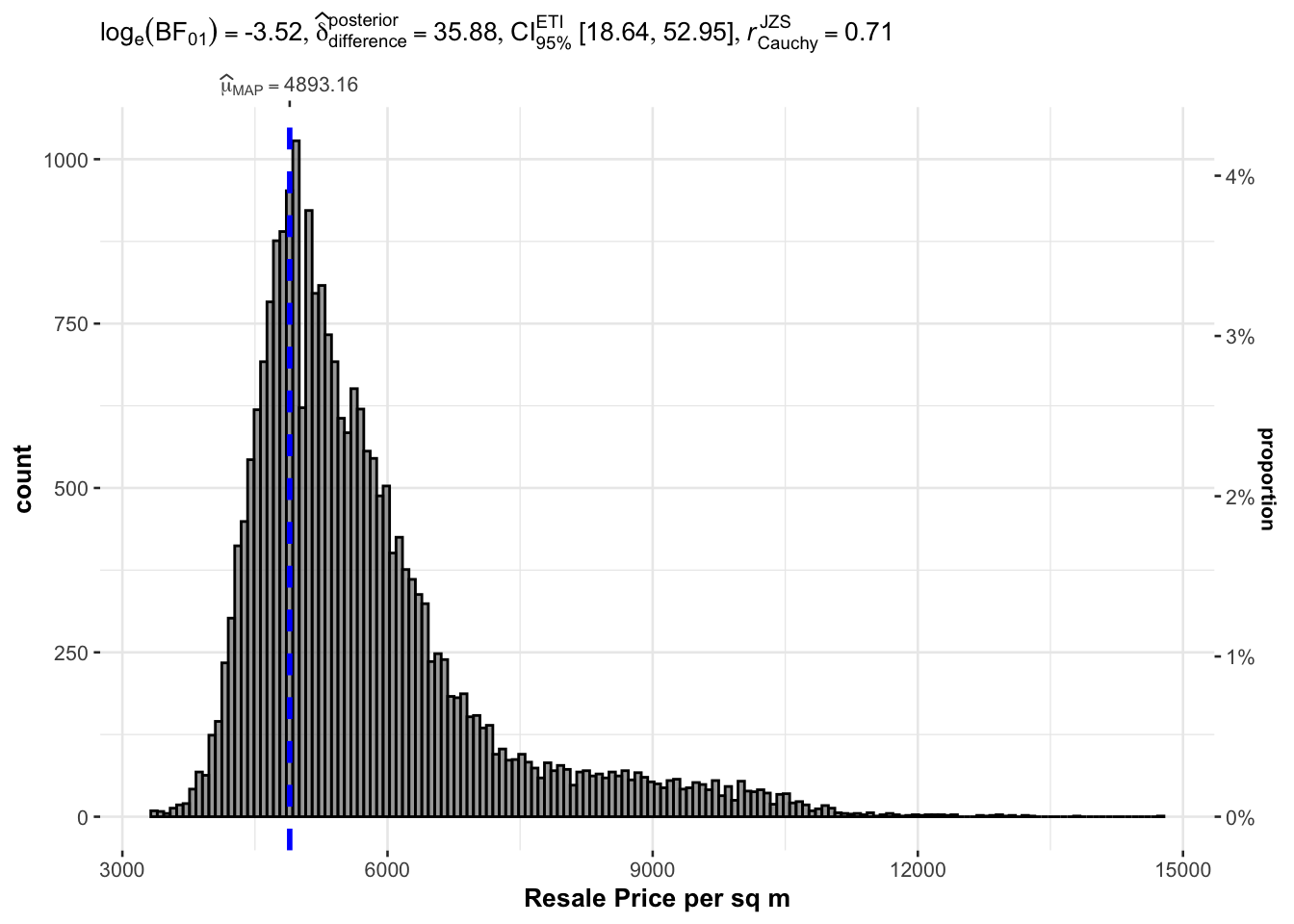
It can be seen that highest proportion of resale price the property around 4.9k per sq meter.
Two sample mean test is done on data of flat_type and pricePerSqm
ggbetweenstats(
  data = data,
  x = flat_type,
  y = pricePerSqm,
  type = "np",
  messages = FALSE
)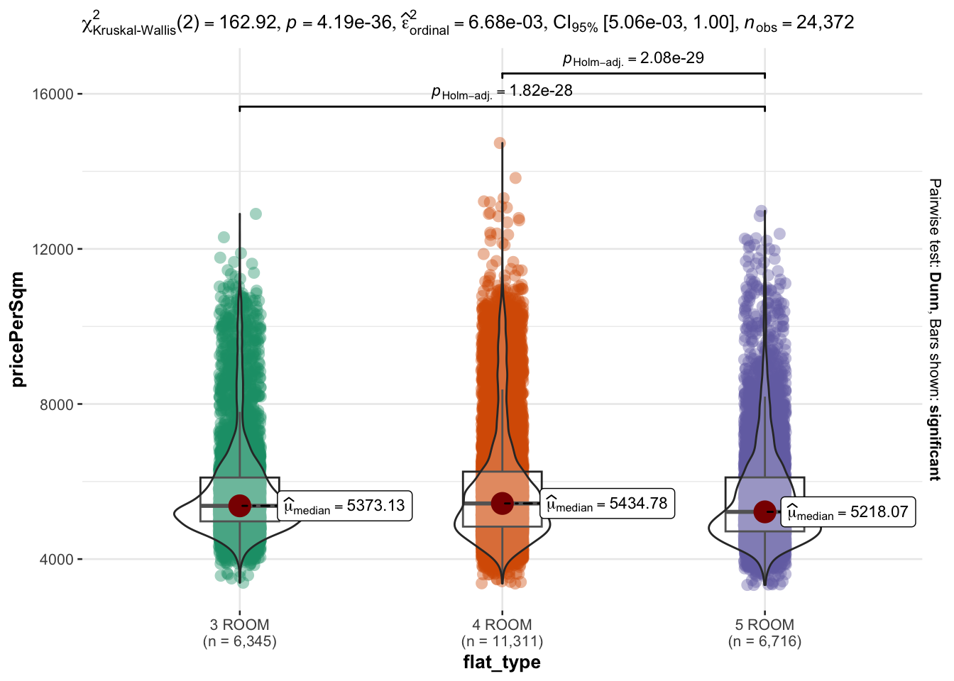
There are slight variation in the price per sq m in different flat types. The median of 3 and 4 rooms are higher than 5 room, it can signify that people prefer 3-4 rooms as compared to 5 rooms, as the demand goes up, the price also goes up along with that. It can show that Singapore has more nuclear family where 3-4 rooms are enough for them.
Visual for One-way ANOVA Test on flat_type and pricePerSqm
ggbetweenstats(
  data = data,
  x = flat_type,
  y = pricePerSqm,
  type = "p",
  mean.ci = TRUE,
  pairwise.comparisons = TRUE,
  pairwise.display = "s",
  p.adjust.method = "fdr",
  messages = FALSE
)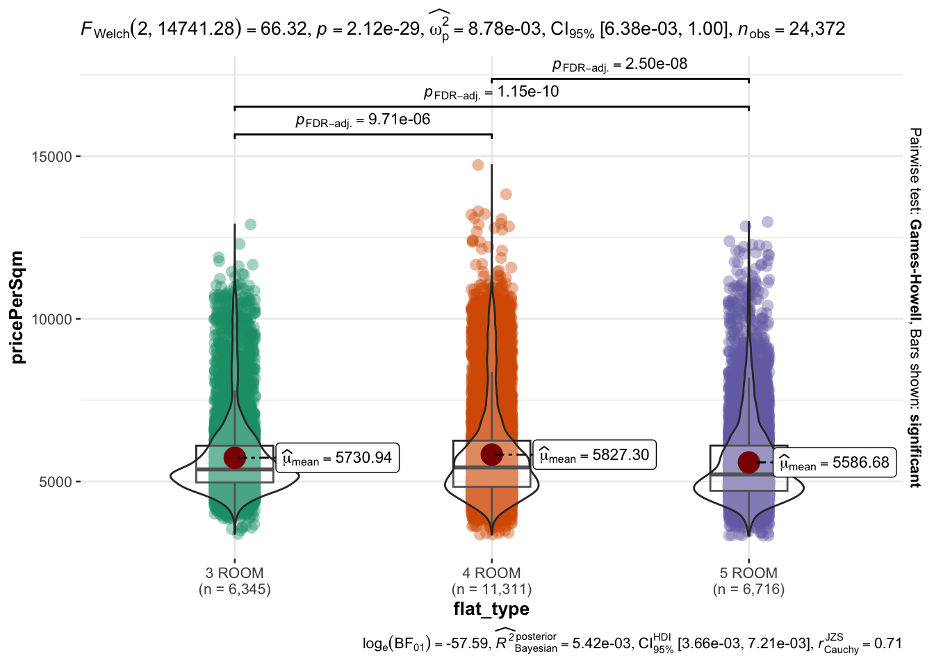
It can be seen that 4 Room are the highest priced whereas 5 room have lower price which can means 5 rooms are lower in demand compared to 3-4 rooms. It can be insightful for analysis on Singapore’s budget and requirements on housing and
ggscatterstats is used to see the relation between pricePerSqm and Remaining Lease.
ggscatterstats(
  data = data,
  x = remainingLease,
  y = pricePerSqm,
  marginal = FALSE,
  )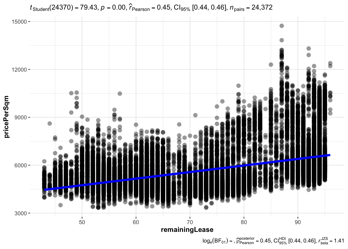
It can be seen that prices have significant variation below 40 and more than 85. As prices are much higher when lease is more than 85 years. The price tend to be lower if the lease is less than 40 years left.
Data mutation before ggbarstats() is used.
data1 <- data %>%
  mutate(remainingLease_bins =
           cut(remainingLease,
               breaks = c(0,40, 60,80, 100))
)ggbarstats(data1,
x = remainingLease_bins,
y = flat_type)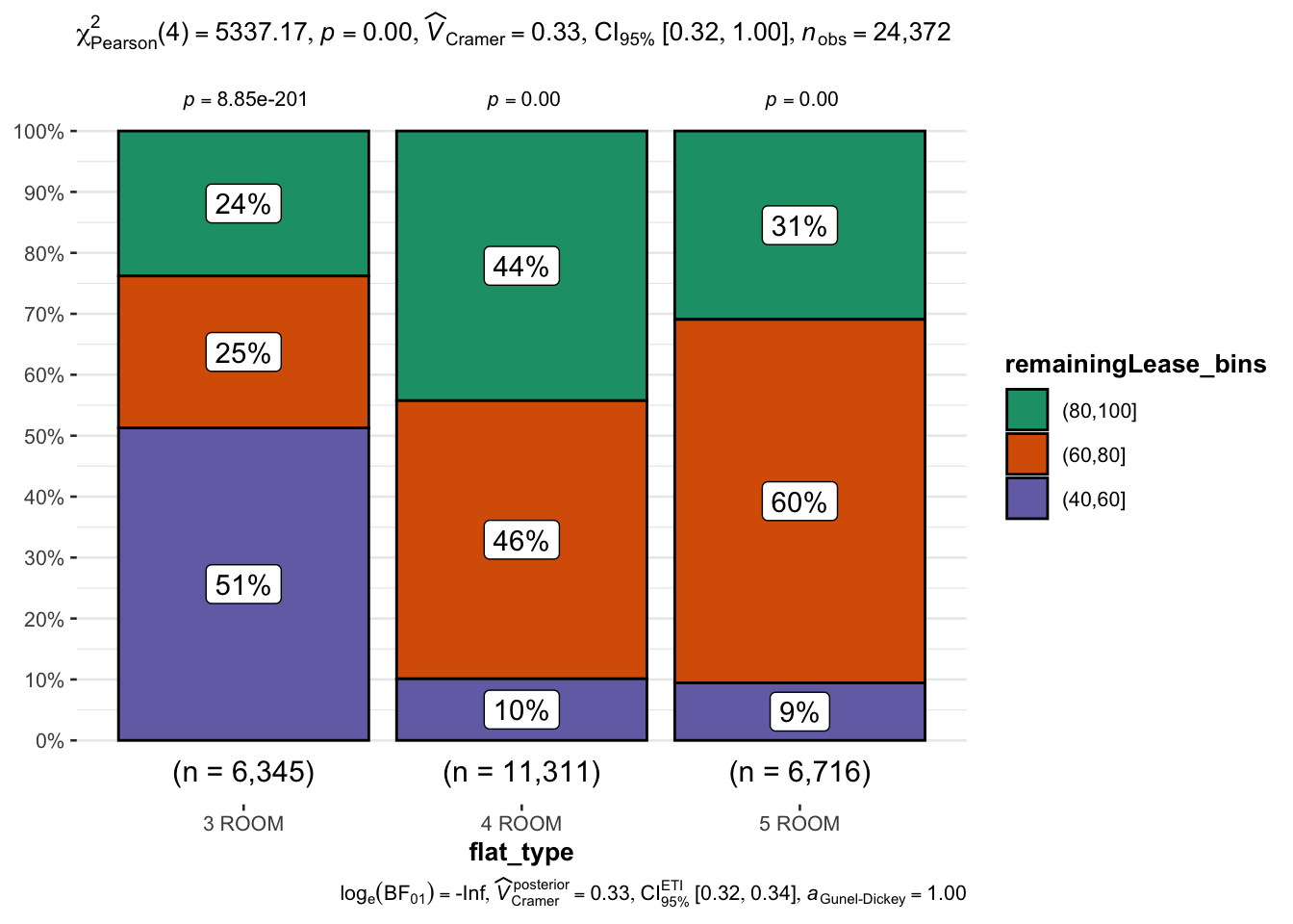
Remaining Lease is divided into 3 categories (i.e. 40-60, 60-80, 80-100).
3 Room have half of the rooms under 40-60 years lease left, i.e. on the lower end of the remaining lease. whereas 4 and 5 Rooms type have good no of years of years left on lease as only 9-10% only have less than 60 years on lease and majority are in 60-100 years of lease.
ggscatterstats(
  data = data,
  x = storey_range,
  y = town,
  marginal = FALSE
) + theme(axis.text.x = element_text(angle = 90, vjust = 0.5, hjust=1))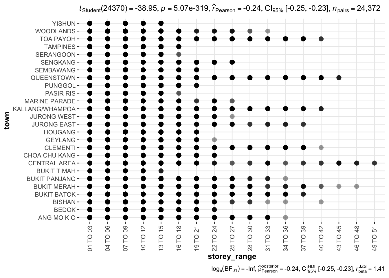
It can be seen here that places like Central Area have higher stories compared to Tampines and Serangoon. This can also impact the resale price.
ggplot(data = data, aes(y = town)) + geom_bar(aes(fill=flat_type))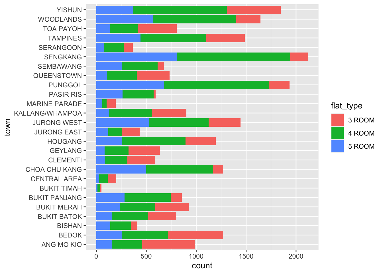
Different town areas have different proportion of room types. 4 room type is quite common in most of the areas.
ggplot(data,
       aes(x = pricePerSqm, y = town, fill =town)) +
  geom_density_ridges(alpha = 0.5) +
  theme_ridges() +
  labs("Price per sq m in different areas of town") +
  theme(legend.position = "none") +
labs(x = "Price per sq m", y = "Area") 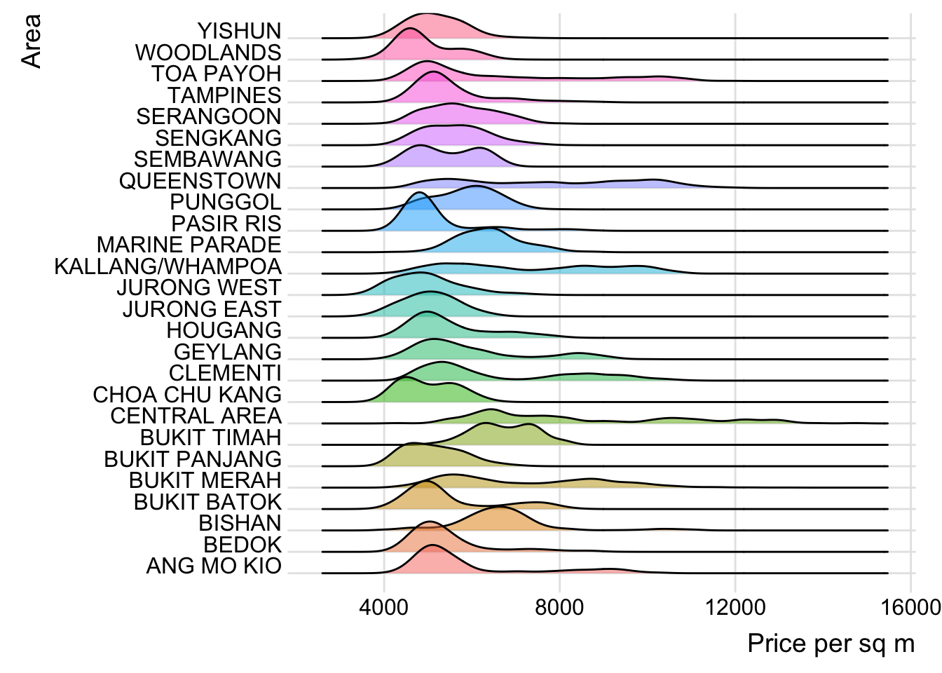
model <- lm(formula = resale_price ~ town + flat_type + storey_range + flat_model + remainingLease,
            data = data)
model
Call:
lm(formula = resale_price ~ town + flat_type + storey_range +
    flat_model + remainingLease, data = data)

Coefficients:
                     (Intercept)                         townBEDOK
                          151789                            -34537
                      townBISHAN                   townBUKIT BATOK
                           97118                            -76741
                 townBUKIT MERAH                 townBUKIT PANJANG
                           81728                           -142853
                 townBUKIT TIMAH                  townCENTRAL AREA
                          158965                             83015
               townCHOA CHU KANG                      townCLEMENTI
                         -159908                              7248
                     townGEYLANG                       townHOUGANG
                           19553                            -79871
                 townJURONG EAST                   townJURONG WEST
                          -87367                           -137464
             townKALLANG/WHAMPOA                 townMARINE PARADE
                           51077                            124002
                   townPASIR RIS                       townPUNGGOL
                          -80850                           -144531
                  townQUEENSTOWN                     townSEMBAWANG
                           76228                           -160337
                    townSENGKANG                     townSERANGOON
                         -154550                              5026
                    townTAMPINES                     townTOA PAYOH
                          -46388                             45546
                   townWOODLANDS                        townYISHUN
                         -145739                           -113317
                 flat_type4 ROOM                   flat_type5 ROOM
                          129210                            280276
            storey_range04 TO 06              storey_range07 TO 09
                           16567                             30470
            storey_range10 TO 12              storey_range13 TO 15
                           36678                             46623
            storey_range16 TO 18              storey_range19 TO 21
                           68597                             95913
            storey_range22 TO 24              storey_range25 TO 27
                          110792                            127522
            storey_range28 TO 30              storey_range31 TO 33
                          166218                            154948
            storey_range34 TO 36              storey_range37 TO 39
                          174175                            180544
            storey_range40 TO 42              storey_range43 TO 45
                          230585                            215197
            storey_range46 TO 48              storey_range49 TO 51
                          351569                            263738
         flat_modelAdjoined flat                    flat_modelDBSS
                            5027                             69916
              flat_modelImproved     flat_modelImproved-Maisonette
                          -65080                            166431
               flat_modelModel A      flat_modelModel A-Maisonette
                          -12830                            153437
              flat_modelModel A2          flat_modelNew Generation
                          -42080                            -26413
     flat_modelPremium Apartment  flat_modelPremium Apartment Loft
                          -12040                            164799
            flat_modelSimplified                flat_modelStandard
                          -54281                            -74066
               flat_modelTerrace                 flat_modelType S1
                          457746                            225949
               flat_modelType S2                    remainingLease
189946 4244 check_c <- check_normality(model)plot(check_c)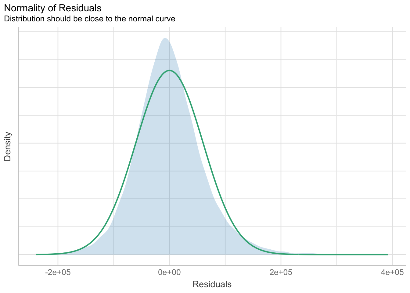
check_h <- check_heteroscedasticity(model)plot(check_h)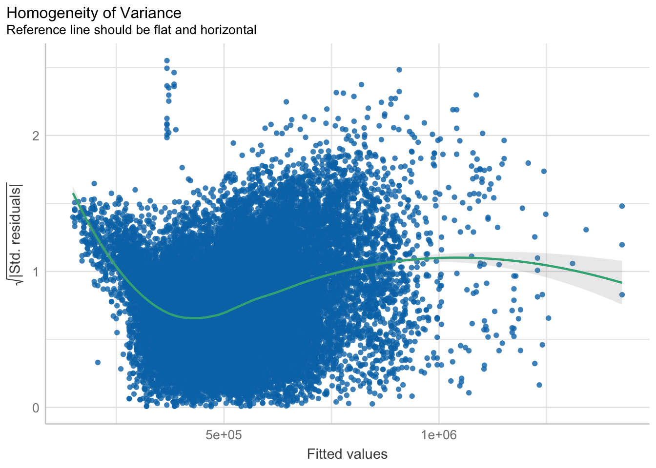
check_model(model)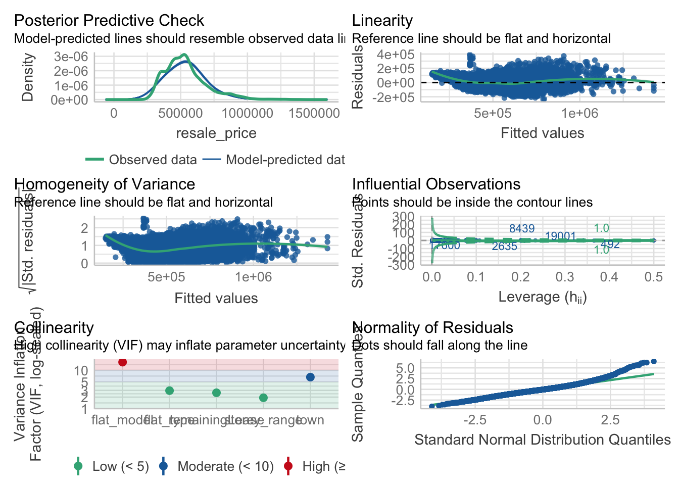
In this task, we used analytical tools to visualise and find features in the data provided.
This visualisation can be helpful in finding patterns for people living in Singapore, how much they are spending on Housing. What’s the demand and supply situation in the current market. How does different parameters affect the market and resale value.
Our key focus was 3/4/5 room type in the current year. Many factors affected the price such as location, storey range, remaining lease, floor area etc.
We used a lot of different tools to visualise different parameters impact on the price.
One single visualisation cannot give a straight forward result. Using many different tools and techniques providing some part of information, we are able to construct the whole picture by combining them.
Overall, it is seen this task that 4 room have higher price and hence highest in demand. 5 rooms are relatively cheaper but with more area, it can be much expensive and not budget-friendly option. 3 rooms will have less area and hence cheaper option but people tend to go more for 4 room which might suggest that people require more 4 room to accommodate their needs.